The Need for Sequence Persistence
Humans do not reset their cognitive state from scratch with every passing second. As you read this sentence, you understand each incoming word based on the context established by the words that preceded it. You do not discard your working memory after every punctuation mark and start your comprehension from zero. Your thoughts possess persistence.
Traditional feed forward neural networks cannot maintain persistence. In a conventional multilayer perceptron or convolutional network, each input sample is processed entirely independently of all previous samples:
This architecture works well for static tasks such as classifying isolated photographs, but it represents a severe shortcoming when analyzing sequential information. Consider an artificial intelligence system trying to predict the next word in a conversational stream, transcribe audio phonemes from continuous speech, or summarize a paragraph of text. To make an accurate prediction at time step , the network must retain context from time steps , and earlier.
Recurrent Neural Networks (commonly abbreviated as RNNs) resolve this challenge. They are neural networks equipped with feedback loops, allowing information to cycle through internal states and persist across sequential transitions.
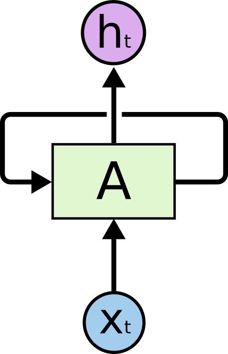
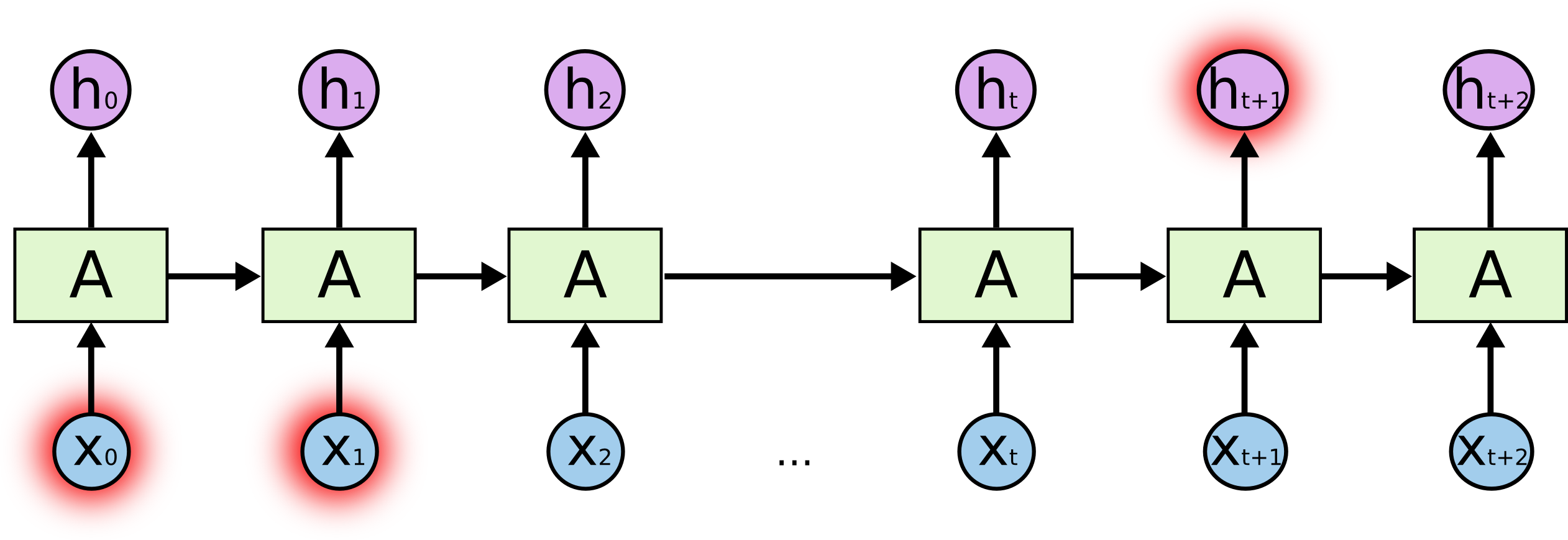
In the diagram above, a modular block of neural network, labeled , receives an input vector at step and emits an output activation vector . The feedback loop allows internal state signals to pass from one processing cycle to the next.
Unrolling Recurrent Neural Networks Through Time
These recurrent feedback loops can initially appear mysterious. However, unrolling the network through time reveals that a recurrent network is simply multiple copies of the exact same neural network layer chained together, with each copy passing its hidden state to its successor:
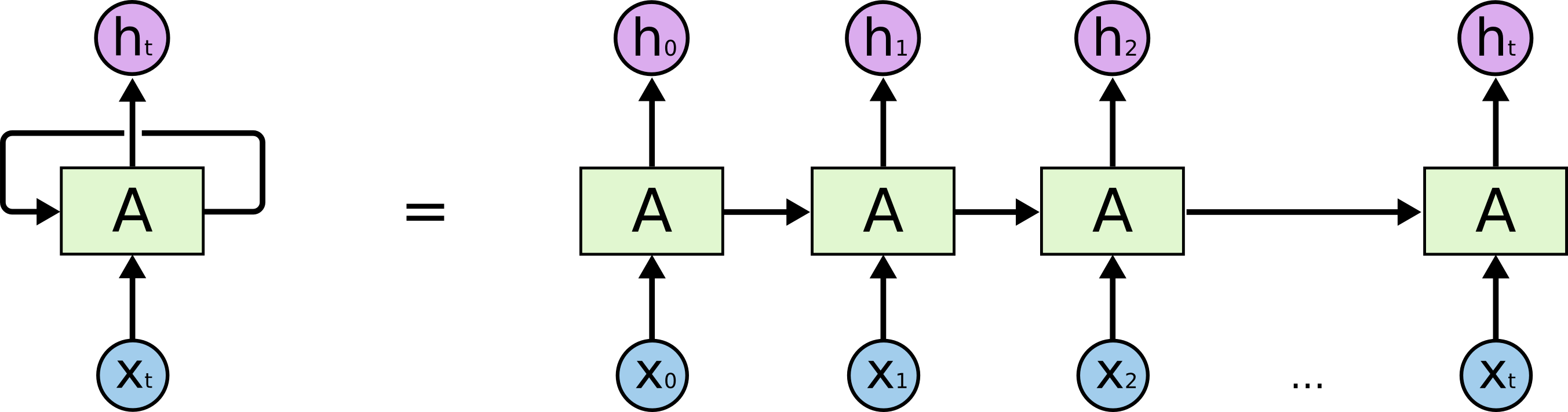
At any individual discrete time step , the standard Elman recurrent network computes its updated hidden state and emission prediction through two matrix transformations:
Here:
- represents the input vector at time step .
- represents the hidden state vector from the previous time step.
- is the parameter weight matrix mapping inputs to hidden states.
- is the shared recurrent parameter weight matrix mapping prior hidden activations to new hidden activations.
- is the hidden state bias vector.
- is the hyperbolic tangent activation function, squashing values into the bounded range .
This unrolled chain structure reveals that recurrent neural networks are fundamentally designed for sequences and ordered lists. They formed the dominant architecture for machine translation, language modeling, and voice recognition for over two decades.
However, standard recurrent networks suffer from a fundamental mathematical flaw that crippled their ability to solve complex, long sequence tasks.
The Dilemma of Long Distance Dependencies
The primary promise of recurrent networks is that they can connect earlier context to a downstream decision. If an autonomous agent reads a continuous text, previous paragraphs should inform current interpretations. Whether a basic RNN can accomplish this depends entirely on the distance between the context and the prediction.
Sometimes, only immediate recent context is required. For example, consider a language model predicting the final word in the phrase:
“The clouds gather in the sky.”
The relevant context word “clouds” sits only four tokens before the blank. Because the distance is minimal, standard recurrent loops easily propagate the contextual signal forward.
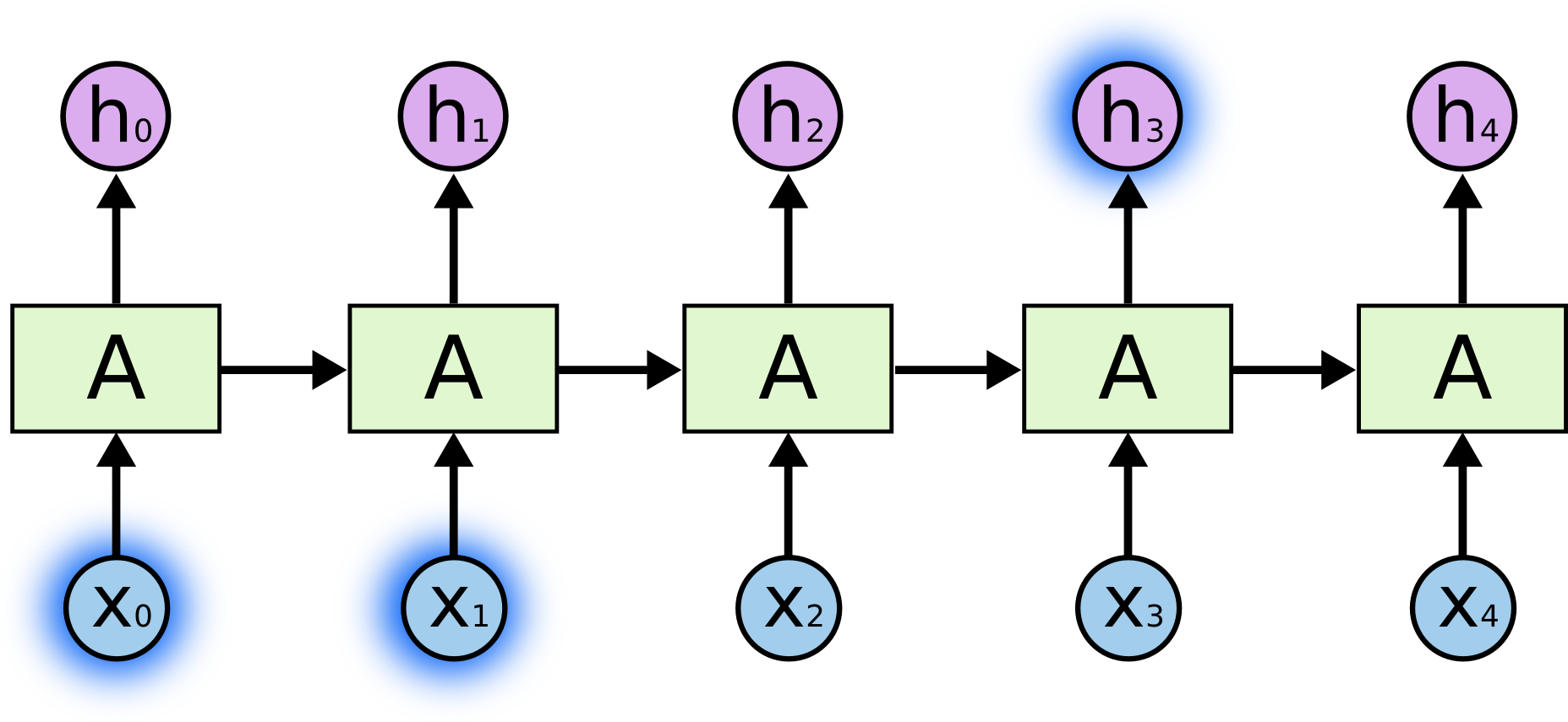
Now consider a case requiring distant contextual memory:
“I spent my early childhood in France… After twenty five years of living overseas, I can still converse fluently in French.”
Recent tokens such as “converse fluently in” suggest that the missing word is the name of a language. But to determine which language, the network must recall the location “France” mentioned dozens of words earlier.
As the temporal distance between the relevant evidence and the target prediction increases, standard recurrent neural networks become mathematically incapable of connecting the information.
The Mathematics of Vanishing and Exploding Gradients
To understand why standard RNNs fail over long distances, we examine how gradients flow backward during training. In Backpropagation Through Time (abbreviated as BPTT), the total loss is calculated across sequence steps, and gradients are propagated backward from step to earlier step :
Let us compute the Jacobian matrix representing the rate of change of state with respect to state :
Notice what occurs across the chain rule product:
This expression contains two critical terms:
- The derivative of the hyperbolic tangent function , which achieves a maximum value of at and decays rapidly toward as activations saturate.
- The recurrent weight matrix multiplied repeatedly by itself times.
If the largest eigenvalue of the recurrent weight matrix is less than (or if activations saturate), the continuous matrix multiplication causes gradient signals to decay exponentially toward zero as they travel backward. Over a modest sequence length of 50 steps, a gradient factor of shrinks to:
The error signal vanishes. The weights in early layers receive virtually zero gradient updates, rendering the network blind to long range historical dependencies.
Conversely, if the eigenvalues exceed , the gradient values explode exponentially, causing numerical instability, arithmetic overflow, and divergence during gradient descent updates.
The Core Architecture of Long Short Term Memory
Long Short Term Memory networks (commonly known as LSTMs) were invented in 1997 by Sepp Hochreiter and Jürgen Schmidhuber specifically to resolve the vanishing gradient problem.
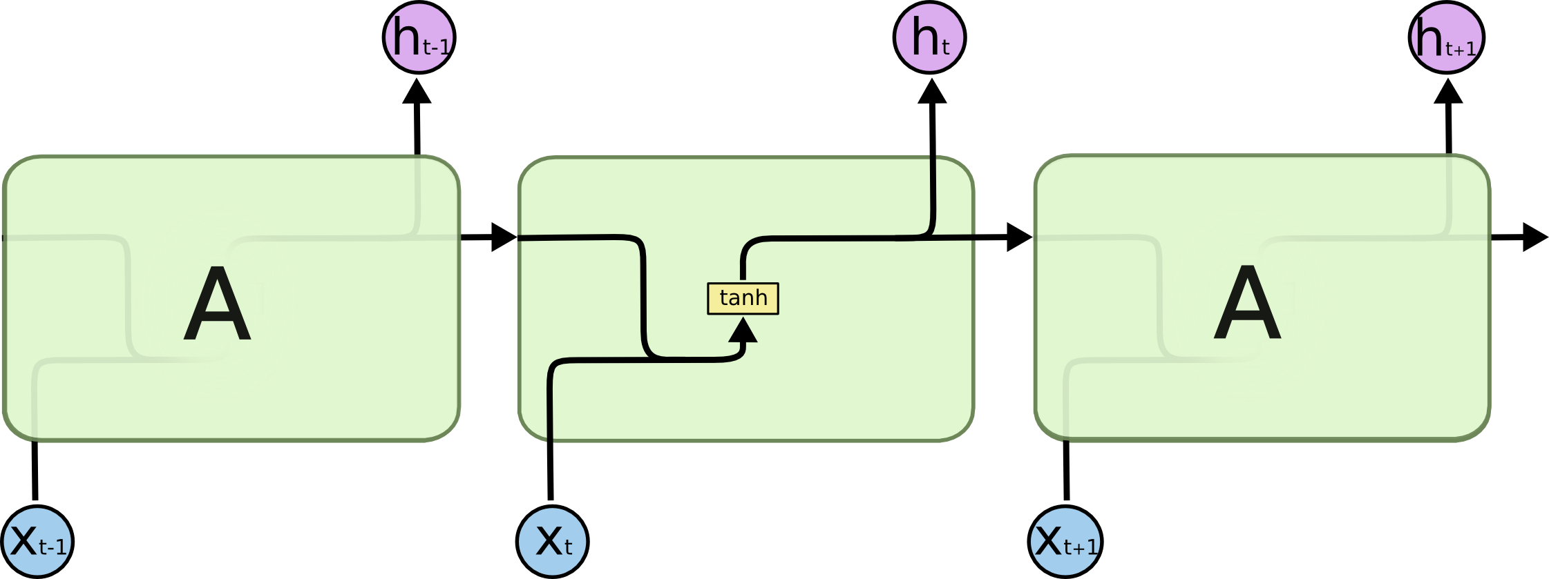
While a standard recurrent neural network contains a simple repeating module with a single hyperbolic tangent layer, an LSTM cell features an intricate internal control structure containing four separate neural network layers that interact in a carefully choreographed manner.
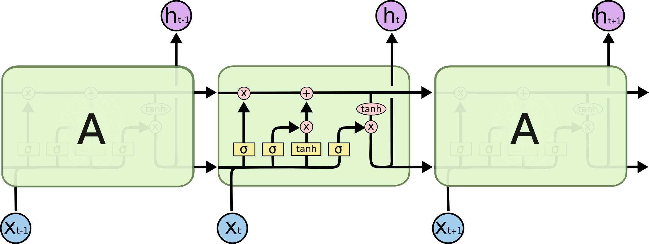
To understand how vectors flow through these interacting layers, let us review the diagram notation guide:

The Constant Error Carousel and Cell State
The central breakthrough of the LSTM is the cell state, denoted as .
The cell state runs straight along the top of the unrolled chain, functioning like a physical conveyor belt or memory bus. Information can travel along this linear channel with minimal multiplicative interference.
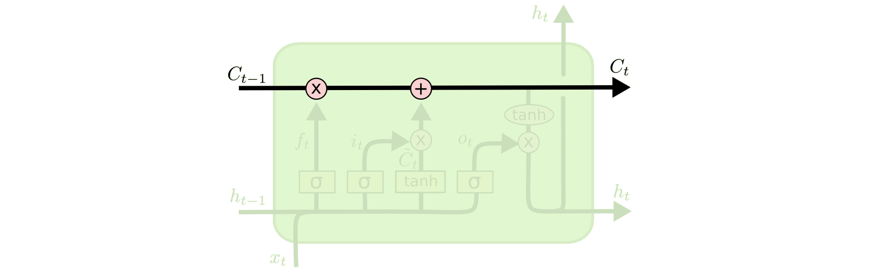
While a standard RNN continuously multiplies hidden states by the weight matrix , the LSTM updates its cell state through linear additions and subtractions. In calculus, the derivative of a linear addition is identity:
By preserving a linear pathway where error signals can flow backward through time without continuous matrix decay, Hochreiter and Schmidhuber created the Constant Error Carousel (CEC), allowing neural networks to maintain memories across hundreds or thousands of steps.
The Role of Gating Layers
To regulate what information enters, remains in, or exits the cell state, LSTMs utilize specialized mechanisms called gates.
A gate consists of an artificial neural network layer with a sigmoid activation function followed by a pointwise elementwise multiplication operation:
The sigmoid function maps any real numbered input into a continuous range between zero and one:
- An activation value of 0 represents a closed gate: “let nothing pass through”.
- An activation value of 1 represents an open gate: “let everything pass through”.
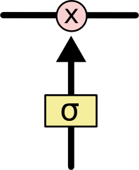
An LSTM contains three fundamental gates:
- The Forget Gate (): Decides what information to purge from the cell state.
- The Input Gate (): Decides what incoming information to write into the cell state.
- The Output Gate (): Decides what filtered version of the cell state to emit as the hidden state .
Step by Step Mathematical Derivation of LSTM Gating
Let us walk through the four mathematical operations executed within an LSTM cell during time step .
Step 1: The Forget Gate Layer
The first decision in the LSTM cell is to identify which information from historical memory should be discarded. This choice is calculated by the forget gate layer:
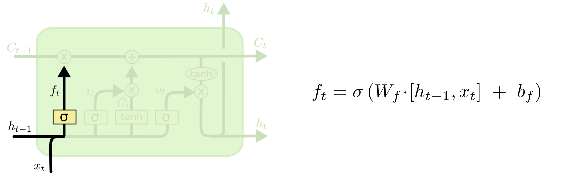
In this equation:
- denotes the concatenation of the previous hidden state vector and the current input vector , producing a combined vector in .
- is the learned forget gate weight matrix.
- is the forget gate bias vector.
- is the sigmoid activation applied element by element.
The resulting vector outputs a value between 0 and 1 for each coordinate in the cell state . For example, in a language model tracking the grammatical gender of a subject, when a new subject noun appears, the forget gate can emit near zero values to purge the gender of the former subject.
Step 2: The Input Gate and Candidate Memory
The second phase determines what new information should be stored in the cell state. This process consists of two coordinated sub steps:
First, the input gate layer applies a sigmoid activation to decide which memory dimensions should be updated:
Second, a candidate state layer applies a hyperbolic tangent activation to synthesize a vector of new candidate values, denoted as , that could be added to the cell state:
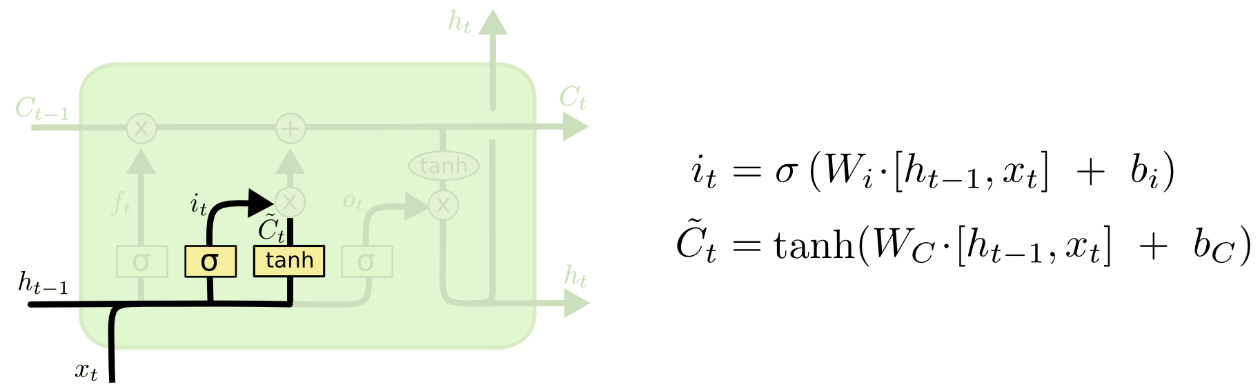
Here:
- and parameterize the input gate.
- and parameterize the candidate memory layer.
- The function bounds candidate values to , preventing unchecked numerical growth.
Together, and determine both what to write and how strongly to write it.
Step 3: Updating the Cell State
We now combine the forget gate decisions and candidate updates to compute the new cell state :
Where represents the Hadamard product (element by element pointwise vector multiplication).
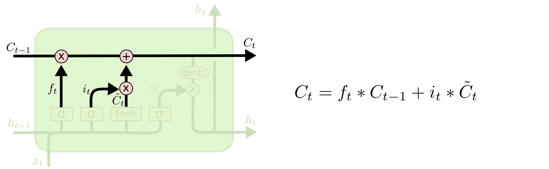
Let us break down the physical meaning of this equation:
- : We scale the old memory state by our forget factors. Any dimension where is cleared; any dimension where is retained intact.
- : We scale our new candidate values by our input gate factors, determining how much fresh evidence to inject.
- The operator: We combine the preserved old state with the new filtered input through simple vector addition.
This additive update is what prevents gradients from vanishing. During backpropagation, the derivative of with respect to contains the additive term :
As long as the network learns to keep the forget gate open (), gradient error signals can backpropagate indefinitely through the sequence without exponential decay.
Step 4: The Output Gate and Hidden State
The final phase produces the outgoing hidden state , which serves two purposes: it is passed to time step as recurrent context, and it is passed to downstream prediction layers (such as a classification head or vocabulary projection).
The output is based on the updated cell state, but passes through an active filter:
First, the output gate layer runs a sigmoid function to decide which parts of the cell state to expose:
Second, we pass the cell state through a hyperbolic tangent function to squash values into the range , and multiply it elementwise by the output gate:
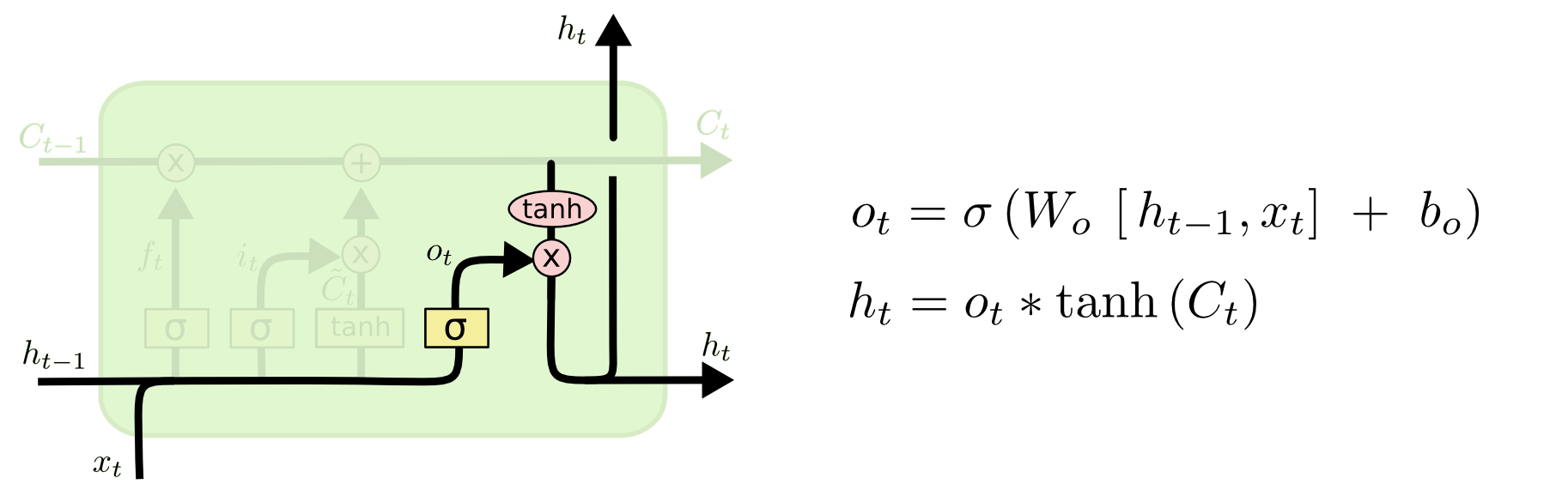
Here:
- and are the output gate parameters.
- represents the visible hidden state emitted at step .
For example, if the cell state remembers that the current grammatical subject is plural, the output gate can expose this property when encountering a verb position so the language model correctly predicts a plural verb form.
Architectural Variants of the Standard LSTM
While the four step formulation described above represents the standard LSTM architecture (often credited to Graves and Schmidhuber), researchers developed several influential architectural variations.
Variant 1: Peephole Connections
Introduced by Felix Gers and Jürgen Schmidhuber in 2000, peephole connections allow the gate layers to inspect the internal cell state directly, rather than relying exclusively on the external hidden state :
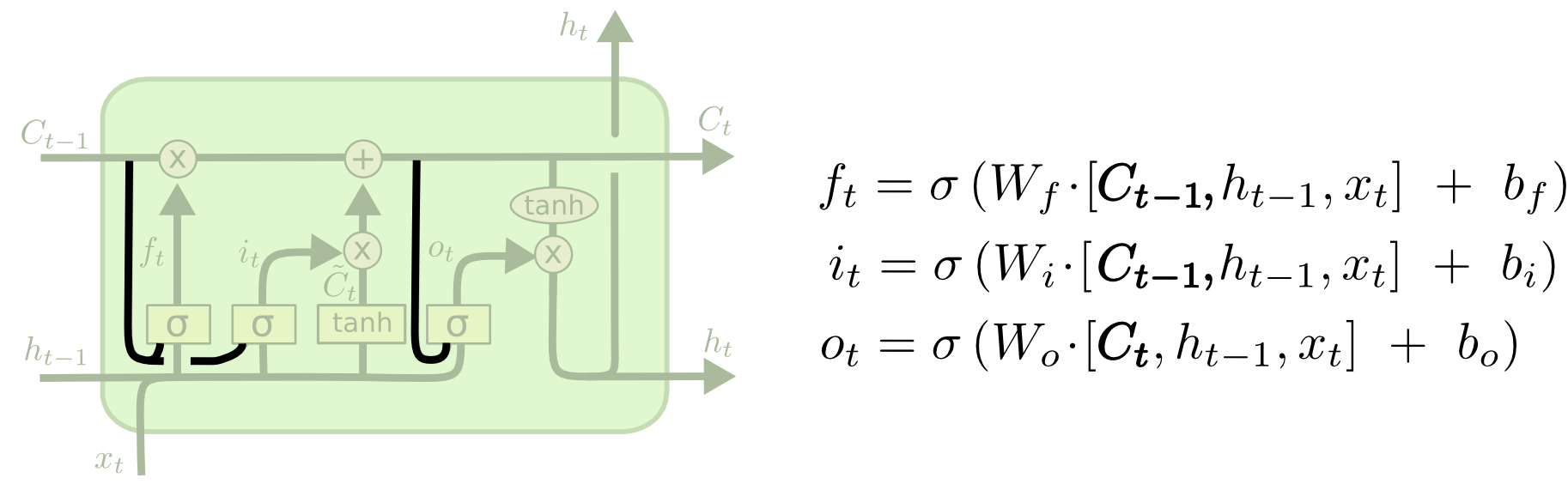
Notice that the forget and input gates inspect the previous cell state , while the output gate inspects the newly updated cell state . Peephole connections allow the network to time intervals and measure sequence durations with higher precision.
Variant 2: Coupled Forget and Input Gates
Another common variation ties the forget decision and input decision together into a single choice. Instead of computing independent gates and , the network only decides what to forget, and automatically fills that freed capacity with new input:
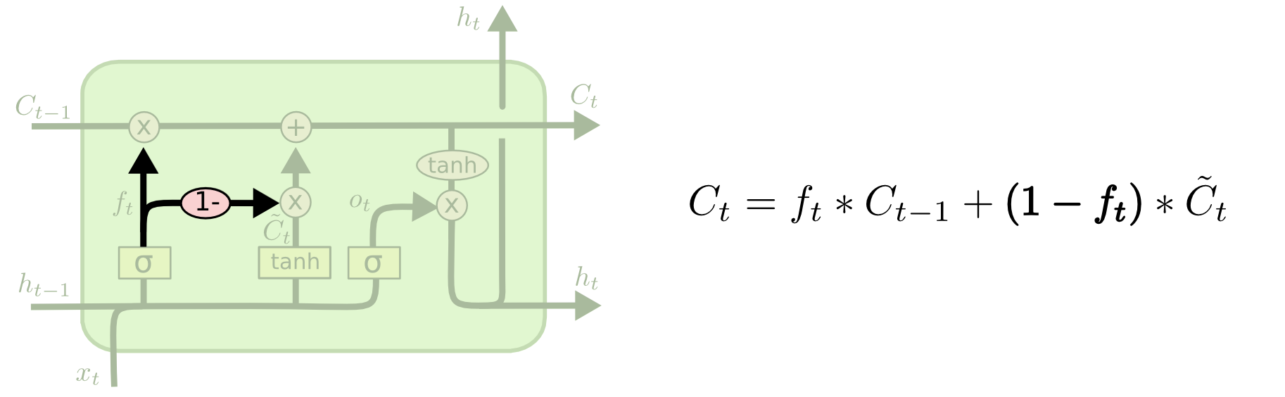
Here, the factor replaces . The network only writes new information to a dimension when it is actively forgetting older information.
Variant 3: The Gated Recurrent Unit (GRU)
Perhaps the most prominent variation is the Gated Recurrent Unit (GRU), introduced by Kyunghyun Cho and colleagues in 2014. The GRU simplifies the LSTM cell by eliminating the separate cell state , merging all memory into a single hidden state :
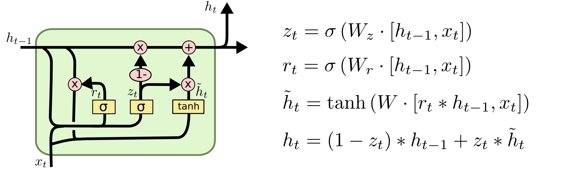
The GRU uses two gates:
- The Reset Gate (): Controls how much previous memory to disregard when computing new candidate states:
- The Update Gate (): Combines the functions of the forget and input gates:
The candidate hidden state is computed by applying the reset gate to the prior hidden state:
The final hidden state interpolation is:
Because the GRU features fewer parameter matrices and requires fewer tensor multiplications per step, it computes faster and requires less memory while achieving competitive performance on many sequential modeling benchmarks.
Summary Comparison of Recurrent Architectures
| Metric / Dimension | Standard RNN | LSTM Cell | Gated Recurrent Unit (GRU) |
|---|---|---|---|
| Introduced By | Rumelhart, Elman (1986, 1990) | Hochreiter, Schmidhuber (1997) | Cho et al. (2014) |
| Persistent States | Single hidden state | Dual states: Cell & Hidden | Single hidden state |
| Gating Mechanisms | None | 3 gates () | 2 gates () |
| Parameter Matrices | 2 () | 4 gate matrices () | 3 gate matrices () |
| Vanishing Gradients | Severe over steps | Minimal over hundreds of steps | Minimal over hundreds of steps |
| Step Execution | Highly lightweight | Moderately heavy | Lightweight to moderate |
From Recurrence to Self Attention: The Evolution to Transformers
For more than a decade, Long Short Term Memory networks powered state of the art sequence applications, from Google Translate to Apple Siri and voice dictation.
However, as dataset sizes surged from millions to billions of tokens, recurrent architectures collided with two fundamental hardware and algorithmic constraints:
1. Sequential Execution Bottleneck
To compute step , an LSTM strictly requires the output of step :
Because step depends on step , recurrent networks cannot parallelize training across sequence positions. Graphics Processing Units (GPUs) and Tensor Processing Units (TPUs) achieve their extraordinary computational throughput by running thousands of matrix multiply operations simultaneously across large parallel cores. When training an RNN, these cores must wait sequentially for each token transition, creating severe training latency.
2. Maximum Signal Path Length
In any recurrent architecture, information from token must travel through physical network steps to reach token . Even with constant error carousels, memory compression remains lossy; squeezing an entire sequence into a fixed dimension hidden vector inevitably creates an information bottleneck.
In 2017, Ashish Vaswani and colleagues published the landmark paper “Attention Is All You Need”, introducing the Transformer architecture. The Transformer completely dismantled recurrence:
- Instead of processing sequentially in operations, the Transformer calculates pairwise relationships across all tokens simultaneously using Self Attention.
- The path length between any two arbitrary tokens in a sequence drops from in an RNN to in a Transformer layer.
- Training is fully parallelized across all sequence tokens, allowing modern models to train across trillions of words.
Understanding recurrent neural networks and LSTM gating equations illuminates why transformers were designed as they were. The core quest of deep learning sequence modeling has always been the same: preserving long distance contextual relationships without losing gradients or hitting hardware limits.
To explore how weights, bias terms, and backpropagation gradients behave in real time, launch our interactive laboratory visualizers below.